POPULAR COURSES
Master Programs





Table of contents:
|
1. Dynamic Array & Next-Gen Lookup Formulas
|
|
2. Advanced Logic & Custom Function Architecture
|
|
3. Complex Text Parsing & Dynamic Range Manipulation
|
|
4. Financial Modeling & Array Vector Processing
|
|
5. Why Choose Apponix? |
|
6. Conclusion |
Mastering advanced Excel formulas is no longer just a nice-to-have skill for office administration; it is a core requirement for high-impact decision-making in modern business.
Whether you are automating financial models, building real-time executive dashboards, or evaluating a Data analytics course in Bangalore to accelerate your career, moving beyond simple SUM and AVERAGE calculations is what sets operational leaders apart.
Modern corporate environments demand dynamic data manipulation, automated error handling, and robust analytical modeling that can handle thousands of rows without manual intervention.
Excel has evolved dramatically with the introduction of its dynamic array engine. The days of dragging formulas down thousands of cells, dealing with broken VLOOKUP references, and writing complex VBA scripts for basic data cleaning are over. Today’s analytics workflows rely on recalculating arrays in real time, declaring localized variables within cells, and creating custom functions natively.
In this guide, we will break down the 20 most critical formulas every analyst, manager, and consultant must master to automate daily reporting and drive data-backed business strategy.
Dynamic Array & Next-Gen Lookup Formulas
The introduction of the dynamic array engine fundamentally transformed how Excel processes data. Instead of writing a formula and manually dragging it across hundreds of rows, dynamic array formulas calculate an entire range of results and "spill" them into neighboring cells automatically.
When modernizing your analytical workflow, mastering a core Advanced Excel functions list focused on dynamic lookup and data extraction is the first step toward building automated, resilient models.
Here are the top five dynamic array and lookup formulas every professional must know:
1. XLOOKUP: The Universal Lookup Engine
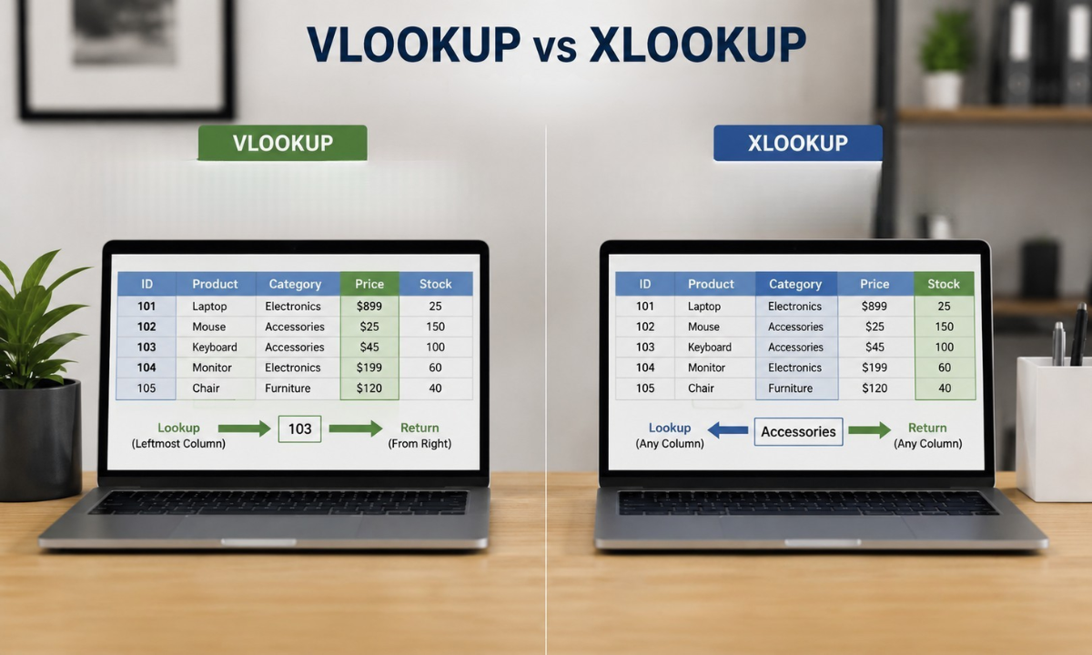
XLOOKUP is the direct, modern replacement for legacy functions like VLOOKUP, HLOOKUP, and LOOKUP. It eliminates the left-to-right lookup restriction, defaults to an exact match, and native error handling prevents broken formulas when columns are inserted or deleted.
Formula Syntax:
=XLOOKUP(lookup_value, lookup_array, return_array, [if_not_found], [match_mode], [search_mode])
Real-World Business Scenario:
You have an employee database where Employee ID is in Column C and Base Salary is in Column A. VLOOKUP fails here because the return column is to the left of the lookup column. XLOOKUP handles this effortlessly while cleanly handling missing IDs.
Practical Example:
=XLOOKUP(E2, C2:C500, A2:A500, "Employee Not Found")
How it works: Searches for the Employee ID in E2 within C2:C500, returns the corresponding salary from A2:A500, and displays "Employee Not Found" if the ID doesn't exist.
2. FILTER: Dynamic Multi-Criteria Data Extraction
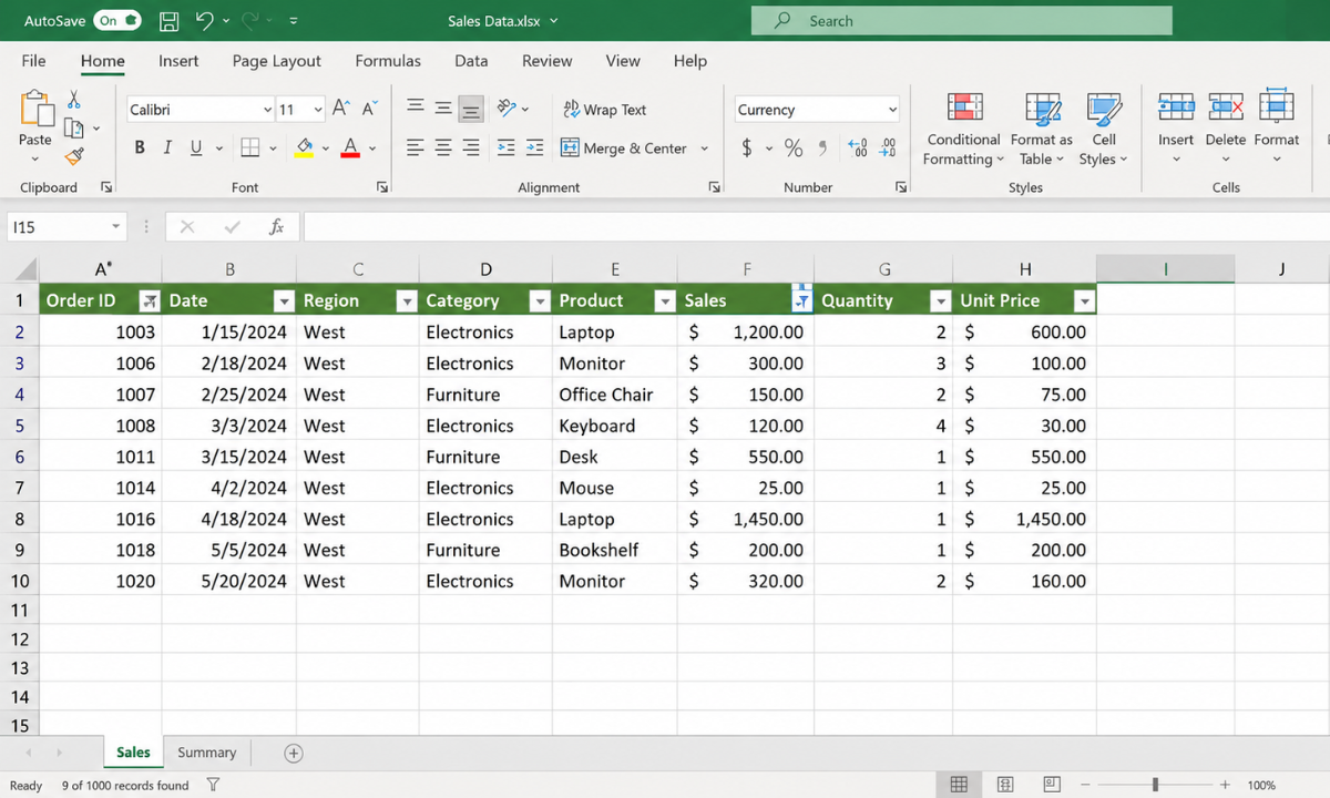
FILTER extracts matching records from a data range based on one or more logical conditions. Unlike traditional Excel filters or Advanced Filter tools, the output automatically updates whenever the source data changes.
Formula Syntax:
=FILTER(array, include, [if_empty])
Real-World Business Scenario:
A sales director needs an automated report showing all active transactions in the "North" region where the deal size exceeds $50,000.
Practical Example:
=FILTER(A2:D100, (B2:B100="North") * (C2:C100>50000), "No Matching Deals")
How it works: Filters the range A2:D100. Multiplication (*) acts as an AND condition, requiring Region (B2:B100) to be "North" and Deal Size (C2:C100) to be greater than 50000. If no records match, it displays "No Matching Deals".
3. SORT / SORTBY: Dynamic Dataset Ordering

SORT and SORTBY allow you to programmatically order a dataset by one or multiple columns without modifying the underlying source table or using manual macros.
Formula Syntax:
=SORT(array, [sort_index], [sort_order], [by_col])
=SORTBY(array, by_array1, [sort_order1], [by_array2], [sort_order2], ...)
Real-World Business Scenario:
You want to display a live dashboard showing the top-performing sales representatives, sorted automatically from highest revenue to lowest.
Practical Example:
=SORT(A2:C50, 3, -1)
How it works: Takes the dataset A2:C50 and sorts it based on the 3rd column (Revenue) in descending order (-1).
Pro Tip: Use SORTBY when you want to sort a visual dataset by a column that is not included in the final output range.
4. UNIQUE: Automated Deduplication

UNIQUE extracts a distinct list of values from a range or array, eliminating duplicate entries instantly. It is especially powerful for creating dynamic drop-down lists and summary tables.
Formula Syntax:
=UNIQUE(array, [by_col], [exactly_once])
Real-World Business Scenario:
You receive a raw transaction log with 10,000 rows and need an updated, distinct list of active product categories for an executive summary
Practical Example:
=UNIQUE(B2:B10000)
How it works: Scans B2:B10000 and spills a single-column list of all distinct product category names without duplicates.
5. SEQUENCE: Dynamic Array Generation
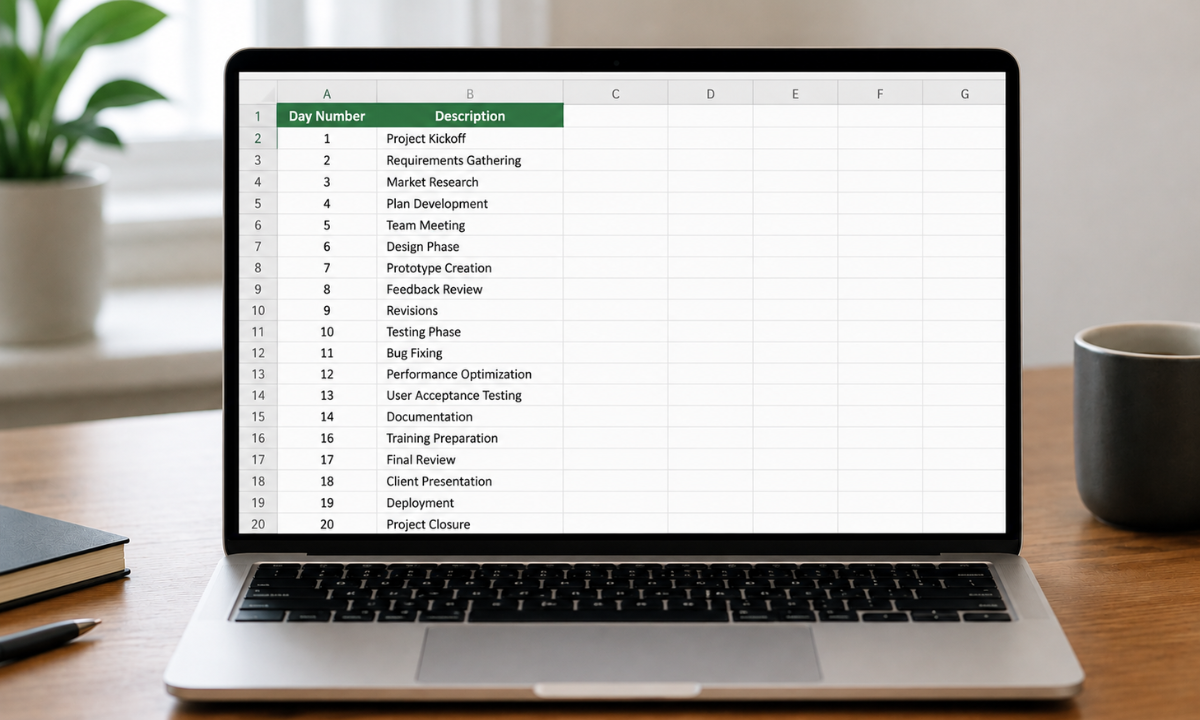
SEQUENCE creates an array of sequential numbers across rows and columns. It is invaluable for generating dynamic index numbers, date series, or matrix indices without manually dragging fill handles.
Formula Syntax:
=SEQUENCE(rows, [columns], [start], [step])
Real-World Business Scenario:
You are building a 12-month financial forecasting model starting in January 2026 and want the schedule dates to generate dynamically.
Practical Example:
=EDATE(DATE(2026, 1, 1), SEQUENCE(1, 12, 0, 1))
How it works: SEQUENCE(1, 12, 0, 1) generates a horizontal array [0, 1, 2, ..., 11]. EDATE then increments the start date Jan 1, 2026 across all 12 months automatically.
Summary Matrix: Dynamic Array Basics
|
Formula |
Primary Use Case |
Output Behavior |
Replaces Legacy Pattern
|
|---|---|---|---|
|
XLOOKUP |
Exact/approximate value retrieval |
Single cell or vector |
VLOOKUP, INDEX/MATCH |
|
FILTER |
Conditional record extraction |
Multi-cell array spill |
Manual AutoFilters, VBA |
|
SORT / SORTBY |
Dynamic dataset ordering |
Multi-cell array spill |
Manual Table Sorting |
|
UNIQUE |
On-the-fly deduplication |
Vector array spill |
Remove Duplicates UI Tool |
|
SEQUENCE |
Programmatic series creation |
Multi-cell vector/matrix |
Manual fill dragging |
Advanced Logic & Custom Function Architecture
Building enterprise-grade financial models and analytical engines requires more than just extracting data; you must process complex logic cleanly and efficiently. As workbooks grow to handle hundreds of thousands of rows, poorly structured formulas can slow down calculation times and make troubleshooting a nightmare.
Leveraging Advanced Excel functions that allow you to define local variables, create reusable logic, and handle multi-criteria conditions is essential for maintaining workbook performance and auditability.
Here are the top five advanced logic and custom function structures used by senior data analysts and financial engineers:
6. LET: Declaring Variables for High-Performance Formulas
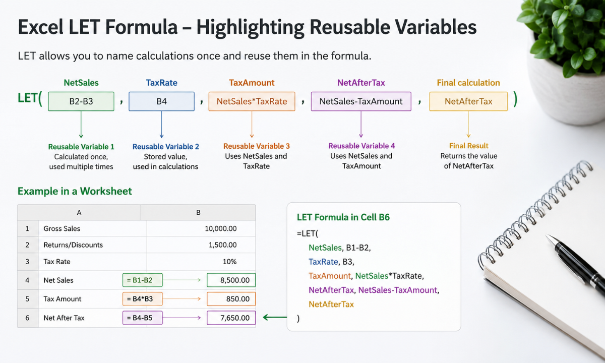
LET allows you to assign names to calculation results and define local variables directly inside a formula. By calculating an intermediate value once and referencing it multiple times, LET dramatically speeds up heavy workbooks and makes complex logic infinitely easier to read and maintain.
Formula Syntax:
=LET(name1, value1, [name2, value2], calculation)
Real-World Business Scenario:
You are calculating performance bonuses where profit margin is evaluated twice in a nested IF statement. Without LET, Excel calculates (Revenue - Cost) / Revenue multiple times for every single row.
Practical Example:
=LET(
rev, A2,
cost, B2,
margin, (rev - cost) / rev,
IF(margin > 0.25, rev * 0.10, rev * 0.02)
)
How it works: Defines rev as A2, cost as B2, and margin as the profit calculation. It then evaluates the IF condition using the pre-calculated margin variable, eliminating redundant calculations.
7. LAMBDA: Creating Custom Functions Without VBA

LAMBDA allows you to turn custom formula logic into reusable user-defined functions without writing a single line of VBA macro code. Once defined in Excel’s Name Manager, you can call your custom function by name anywhere in the workbook.
Formula Syntax:
=LAMBDA([parameter1, parameter2, ...], calculation)
Real-World Business Scenario:
Your organization uses a specific, complex tax-adjusted revenue formula across multiple financial modeling sheets: Revenue * (1 - Tax Rate) * (1 - Discount). Instead of retyping this formula across dozens of cells, you create a standard function named NetTaxRevenue.
Practical Example:
In the Name Manager, define NetTaxRevenue as:
=LAMBDA(rev, tax, disc, rev * (1 - tax) * (1 - disc))
In your worksheet, simply call:
=NetTaxRevenue(A2, 0.21, 0.05)
How it works: Passes cell A2 as revenue, 21% as tax, and 5% as discount directly into your custom LAMBDA formula.
8. SUMIFS: Multi-Criteria Conditional Summation
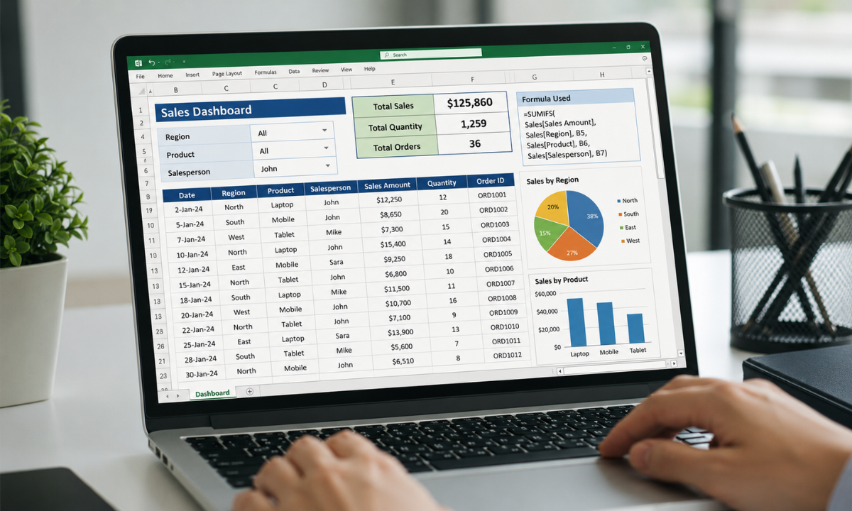
SUMIFS is the primary workhorse for financial reconciliation, budget vs. actual variance analysis, and management reporting. It aggregates values in a target range only when all specified criteria are met.
Formula Syntax:
=SUMIFS(sum_range, criteria_range1, criteria1, [criteria_range2, criteria2], ...)
Real-World Business Scenario:
A corporate controller needs total sales for the "Enterprise" client segment within the "Q3" fiscal period for the "EMEA" region.
Practical Example:
=SUMIFS(D2:D1000, A2:A1000, "Enterprise", B2:B1000, "Q3", C2:C1000, "EMEA")
How it works: Sums values in D2:D1000 (Sales Amount) only where A2:A1000 equals "Enterprise", B2:B1000 equals "Q3", and C2:C1000 equals "EMEA".
9. COUNTIFS: Multi-Condition Operational Auditing
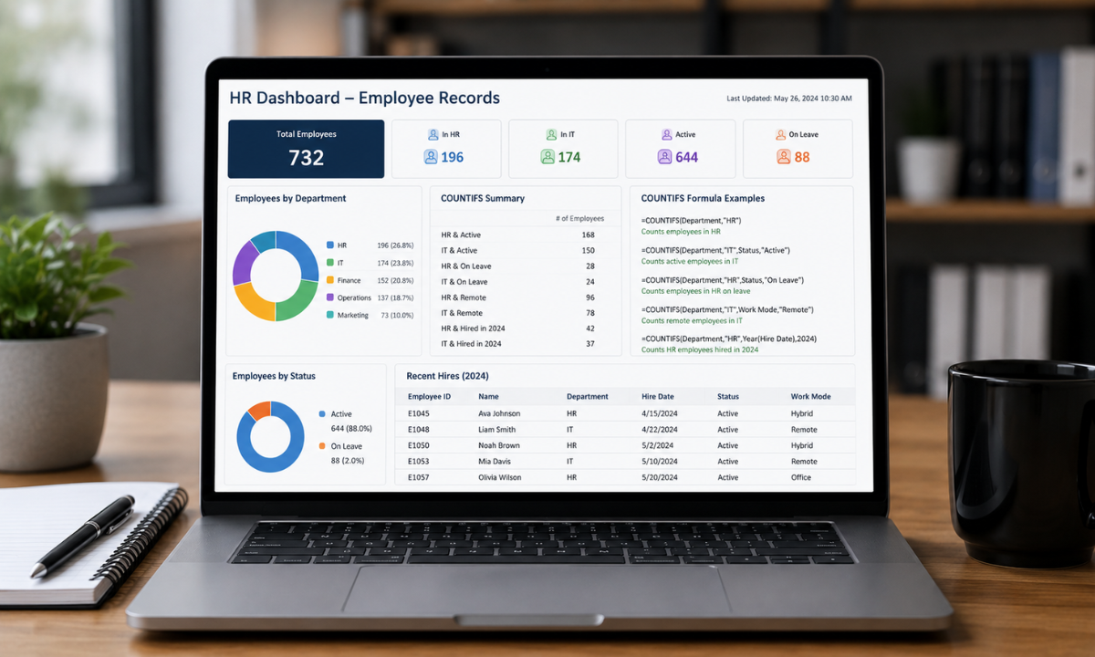
COUNTIFS tallies the number of rows that satisfy multiple logical tests. It is widely used in SLA compliance monitoring, inventory tracking, and HR analytics.
Formula Syntax:
=COUNTIFS(criteria_range1, criteria1, [criteria_range2, criteria2], ...)
Real-World Business Scenario:
An IT operations manager needs to count all open support tickets categorized as "Critical" priority that have been pending for longer than 24 hours.
Practical Example:
=COUNTIFS(B2:B500, "Critical", C2:C500, "Open", D2:D500, ">24")
How it works: Evaluates range B2:B500 for "Critical", C2:C500 for "Open", and D2:D500 for ticket age greater than 24 hours, returning the exact number of matching breach risks.
10. IFERROR + INDEX/MATCH: Safe Legacy Matrix Lookups
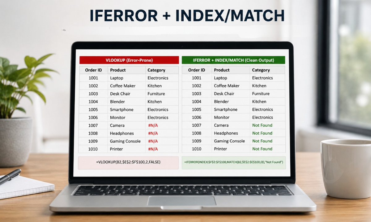
While XLOOKUP is preferred in modern Excel versions, INDEX/MATCH combined with IFERROR remains the gold standard for legacy environment compatibility and complex two-way matrix lookups across rows and columns simultaneously.
Formula Syntax:
=IFERROR(INDEX(return_range, MATCH(lookup_row_val, row_range, 0), MATCH(lookup_col_val, col_range, 0)), "Fallback Value")
Real-World Business Scenario:
You are pulling financial metric figures from a historic cross-tabulation table where both row headers (Fiscal Year) and column headers (Department) are dynamic, while ensuring old Excel versions do not throw raw #N/A errors.
Practical Example:
=IFERROR(INDEX(B2:G100, MATCH(I2, A2:A100, 0), MATCH(J1, B1:G1, 0)), "Data Unavailable")
How it works: MATCH(I2, A2:A100, 0) finds the target row for Year I2. MATCH(J1, B1:G1, 0) finds the target column for Department J1. INDEX retrieves the intersecting cell value. If either match fails, IFERROR neatly outputs "Data Unavailable".
Logic & Performance Reference Matrix
|
Formula / Pattern |
Primary Technical Advantage |
Optimization Impact
|
|---|---|---|
|
LET |
Eliminates redundant inner calculations |
High (reduces calculation time up to 80% in large sheets) |
|
LAMBDA |
Standardizes business logic enterprise-wide |
Medium (eliminates formula copy-paste errors) |
|
SUMIFS |
Multi-attribute aggregation |
Essential (foundational for corporate reporting) |
|
COUNTIFS |
Multi-condition frequency tracking |
Essential (foundational for compliance auditing) |
|
IFERROR + INDEX/MATCH |
Two-way grid lookup + error masking |
High (ensures model stability in legacy Excel builds) |
Complex Text Parsing & Dynamic Range Manipulation
Data arriving from external ERPs, legacy databases, or web exports is rarely clean. Analysts often spend hours manually splitting strings, reordering columns, or rebuilding broken sheet references when monthly financial tabs update.
Mastering advanced text processing and flexible range references turns messy raw files into automated, self-healing data pipelines. To help you master these techniques, here are five essential Excel formulas with examples designed for complex string parsing and flexible range references:
11. TEXTJOIN: Delimited String Concatenation
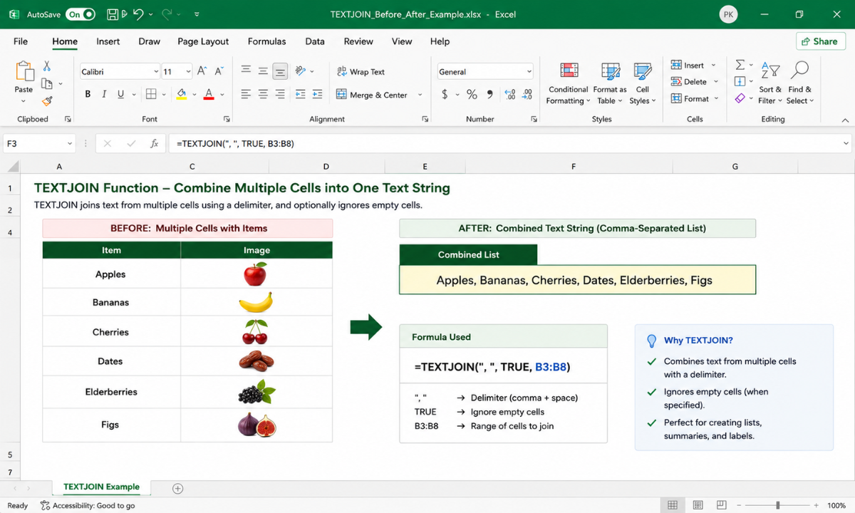
TEXTJOIN merges text strings from multiple cells or ranges using a specified delimiter (such as a comma, space, or hyphen) while automatically skipping empty cells. It eliminates the need for endless & concatenation chains.
Formula Syntax:
=TEXTJOIN(delimiter, ignore_empty, text1, [text2], ...)
Real-World Business Scenario:
An HR coordinator needs to generate a consolidated, comma-separated list of completed compliance certifications for an employee from a row that contains empty cells for uncompleted modules.
Practical Example:
=TEXTJOIN(", ", TRUE, B2:G2)
How it works: Concatenates all non-empty text strings across range B2:G2, separates each entry with a comma and space (", "), and skips blank cells because ignore_empty is set to TRUE.
12. TEXTBEFORE / TEXTAFTER: Precision String Extraction
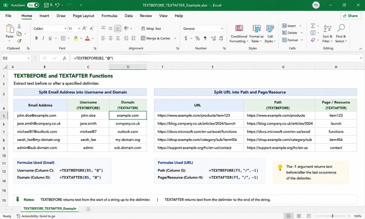
TEXTBEFORE and TEXTAFTER extract portions of a text string surrounding a specific character or delimiter. These functions replace cumbersome combinations of MID, LEFT, RIGHT, SEARCH, and LEN.
Formula Syntax:
=TEXTBEFORE(text, delimiter, [instance_num], [match_mode], [match_end], [if_not_found])
=TEXTAFTER(text, delimiter, [instance_num], [match_mode], [match_end], [if_not_found])
Real-World Business Scenario:
You have a column containing corporate email addresses (john.doe@enterprise.com) and need to extract both the employee's full name before the @ symbol and the corporate domain name after it into separate reporting columns.
Practical Example:
=TEXTBEFORE(A2, "@")
=TEXTAFTER(A2, "@")
How it works: =TEXTBEFORE(A2, "@") extracts "john.doe". =TEXTAFTER(A2, "@") extracts "enterprise.com". You can also specify instance numbers if a delimiter appears multiple times in a string (e.g., slashes in URL paths).
13. INDIRECT: Dynamic Sheet and Range Referencing
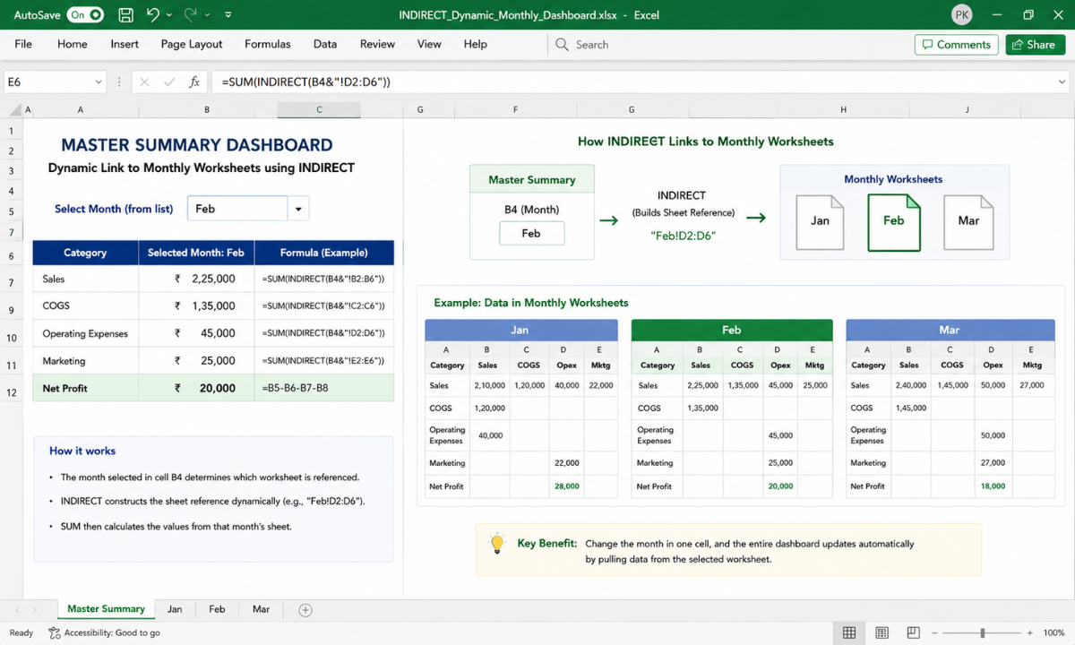
INDIRECT converts a plain text string into a valid Excel cell reference. It allows you to build formulas that dynamically point to different worksheets or named ranges based on user selection or cell values.
Formula Syntax:
=INDIRECT(ref_text, [a1])
Real-World Business Scenario:
A financial analyst maintains twelve monthly sheets named "Jan", "Feb", "Mar", and so on. In a master summary tab, cell A2 contains the month name "Feb". The analyst wants to pull total revenue from cell R50 of whichever month tab is specified in A2 without manually editing the sheet link every month.
Practical Example:
=INDIRECT("'" & A2 & "'!R50")
How it works: Builds the text string 'Feb'!R50 and evaluates it as a live cell reference, retrieving the revenue figure directly from cell R50 of the "Feb" worksheet.
14. OFFSET: Volatile Dynamic Range Construction
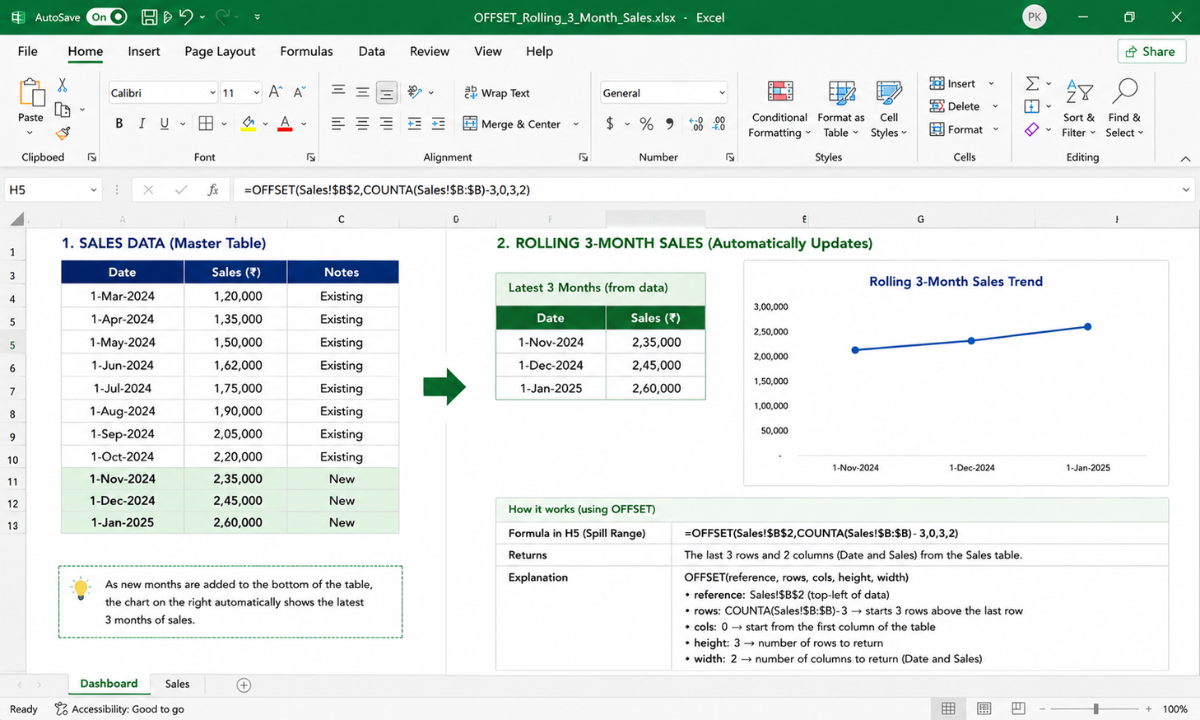
OFFSET generates a reference to a cell or range that is a specified number of rows and columns away from a starting cell. It is widely used for creating dynamic ranges in interactive charts and rolling average calculations.
Formula Syntax:
=OFFSET(reference, rows, cols, [height], [width])
Real-World Business Scenario:
A supply chain manager needs a trailing 3-month average inventory figure that automatically shifts forward every time a new monthly row is appended to the bottom of a historical log table.
Practical Example:
=AVERAGE(OFFSET(B1, COUNTA(B:B)-1, 0, -3, 1))
How it works: COUNTA(B: B)-1 locates the last populated row in Column B. OFFSET starts at that bottom cell and creates a range that is 3 rows high going upward (-3) and 1 column wide. AVERAGE then calculates the mean of those three most recent data points.
Performance Note: OFFSET is a volatile function: it recalculates every time any change is made in the entire workbook. Use OFFSET sparingly in large enterprise models, or replace it with non-volatile dynamic array alternatives like INDEX ranges or CHOOSEROWS.
15. CHOOSECOLS / CHOOSEROWS: Array Subset Selection
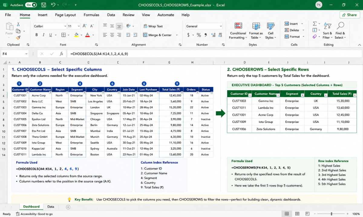
CHOOSECOLS and CHOOSEROWS extract specific columns or rows from a multi-column array without altering or copying the source dataset. They are essential when using FILTER or XLOOKUP over wide data matrices where you only want to display non-adjacent columns in your final report.
Formula Syntax:
=CHOOSECOLS(array, col_num1, [col_num2], ...)
=CHOOSEROWS(array, row_num1, [row_num2], ...)
Real-World Business Scenario:
You are filtering a 15-column master customer table using the FILTER function. However, your executive view should only display Column 1 (Customer Name), Column 4 (Account Manager), and Column 12 (YTD Sales).
Practical Example:
=CHOOSECOLS(FILTER(A2:O500, C2:C500="Active"), 1, 4, 12
How it works: FILTER extracts all 15 columns for rows marked "Active". CHOOSECOLS wraps that dynamic array and isolates only the 1st, 4th, and 12th columns for display.
Text & Range Manipulation Summary
|
Formula |
Function Category |
Primary Operational Problem Solved
|
|---|---|---|
|
TEXTJOIN |
String Parsing |
Merging cell lists with delimiters while skipping empty cells |
|
TEXTBEFORE / TEXTAFTER |
String Parsing |
Substring extraction without nested LEFT/MID/SEARCH logic |
|
INDIRECT |
Dynamic Referencing |
Constructing flexible sheet and range paths from cell text |
|
OFFSET |
Range Creation |
Building shifting references for rolling calculations and charts |
|
CHOOSECOLS / CHOOSEROWS |
Array Manipulation |
Cherry-picking non-adjacent columns/rows from array spills |
Financial Modeling & Array Vector Processing
When evaluating capital investments, forecasting project timelines, or performing matrix calculations, standard arithmetic functions fall short. Corporate finance leads, investment analysts, and project managers require mathematical precision that accounts for real-world irregularities such as non-periodic cash flows, regional working schedules, and multi-dimensional array vectoring.
Mastering advanced financial and array-helper Excel formulas for professionals allows you to perform institutional-grade valuation modeling and process complex array vectors directly in memory.
Here are the final five essential formulas to complete your advanced toolkit:
16. XNPV: Precise Net Present Value for Irregular Cash Flows
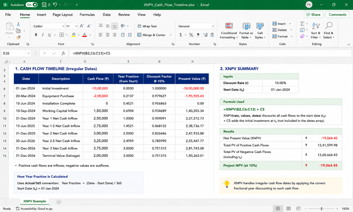
Unlike standard NPV (which assumes cash flows occur at equal, periodic intervals like the end of every year), XNPV calculates the net present value of an investment using exact calendar dates for each cash flow.
Formula Syntax:
=XNPV(rate, values, dates)
Real-World Business Scenario:
A corporate development team is evaluating an acquisition where capital injections and earned payouts occur on specific, irregular milestone dates across a in ba3-year timeline.
Practical Example:
=XNPV(0.08, B2:B6, C2:C6)
How it works: Applies an 8% annual discount rate (0.08) to cash flows in B2:B6 based on the exact transaction dates listed in C2:C6.
17. XIRR: Internal Rate of Return for Real-World Schedules
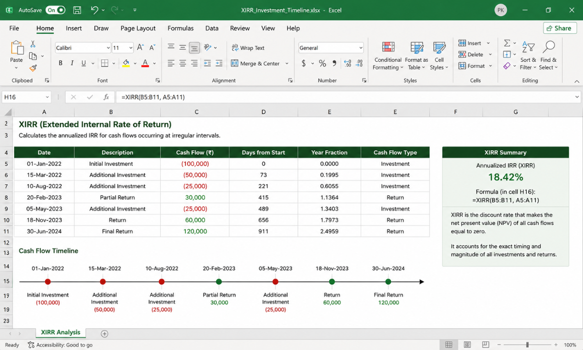
XIRR computes the annualized internal rate of return for a series of cash flows that arrive on irregular dates. It is the gold standard in private equity, venture capital, and corporate treasury for evaluating portfolio returns.
Formula Syntax:
=XIRR(values, dates, [guess])
Real-World Business Scenario:
A venture capital firm tracks an initial startup investment followed by multiple follow-on funding rounds and partial exit distributions made on random dates over five years.
Practical Example:
=XIRR(B2:B10, C2:C10)
How it works: Evaluates the vector of negative cash flows (investments) and positive cash flows (returns) in B2:B10 against their exact date stamps in C2:C10 to return the precise effective annualized return percentage.
18. NETWORKDAYS.INTL: Workday Calculations with Custom Schedules
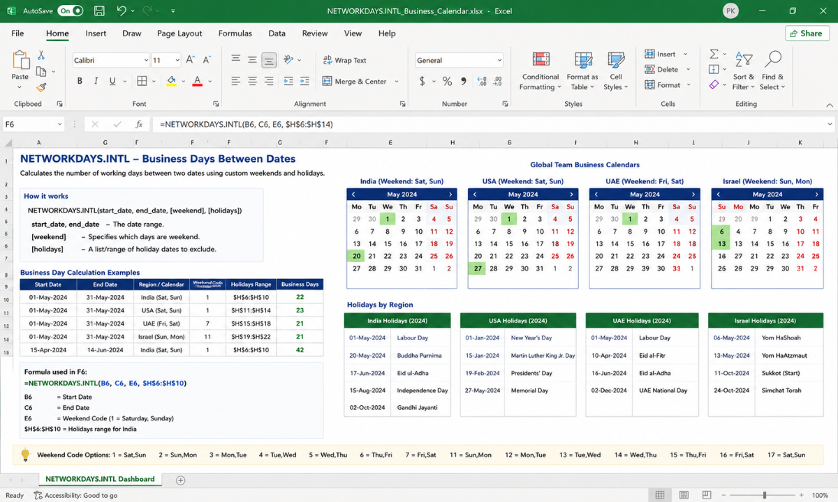
NETWORKDAYS.INTL calculates the total number of working days between two dates, automatically excluding weekends and specified company holidays. The.INTL variant allows you to define custom weekend schedules for global teams operating outside standard Saturday/Sunday weekends.
Formula Syntax:
=NETWORKDAYS.INTL(start_date, end_date, [weekend], [holidays])
Real-World Business Scenario:
A global project manager needs to calculate SLA completion time for a team based in Dubai, where the official weekend is Friday and Saturday rather than Saturday and Sunday.
Practical Example:
=NETWORKDAYS.INTL(A2, B2, 7, Holidays!A2:A15)
Calculates working days between Start Date (A2) and End Date (B2). Parameter 7 sets the weekend strictly to Friday and Saturday, while subtracting any statutory dates listed in Holidays!A2:A15.
19. SUMPRODUCT: Multi-Vector Array Multiplication & Aggregation
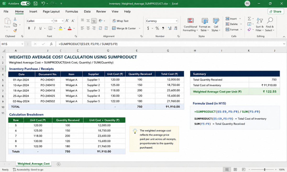
SUMPRODUCT multiplies corresponding components in two or more equal-sized arrays and returns the sum of those products. It is invaluable for weighted averages, risk scoring, and conditional evaluations without requiring helper columns.
Formula Syntax:
=SUMPRODUCT(array1, [array2], [array3], ...)
Real-World Business Scenario:
A procurement manager wants to calculate the Weighted Average Unit Price of inventory across multiple warehouse orders without adding a separate "Total Cost" column for every row.
Practical Example:
=SUMPRODUCT(B2:B50, C2:C50) / SUM(C2:C50)
How it works: SUMPRODUCT(B2:B50, C2:C50) multiplies Unit Price (B2:B50) by Quantity (C2:C50) for each row and sums the result. Dividing by =SUM(C2:C50) yields the exact weighted average unit cost instantly.
20. MAP / REDUCE: Advanced Array Transformation Helpers
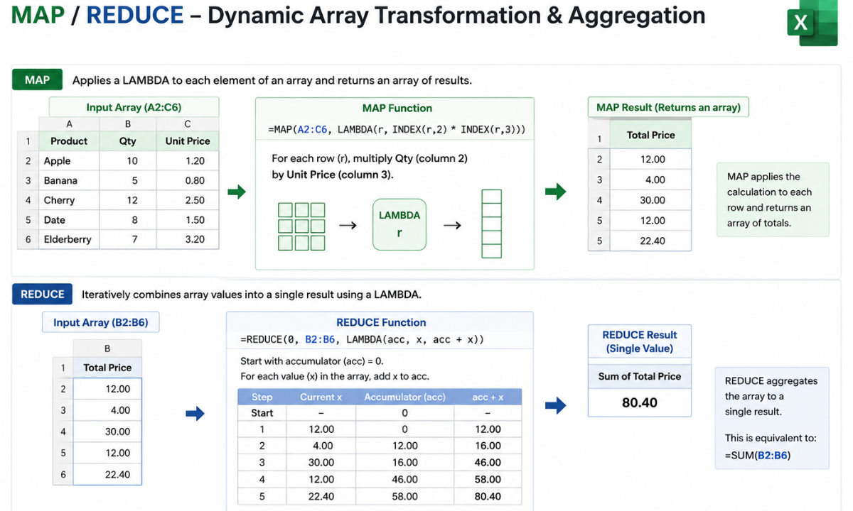
MAP and REDUCE are advanced Lambda helper functions designed for custom vector processing. MAP applies a LAMBDA function row-by-row across an entire array, returning a transformed dynamic array. REDUCE iterates through an array and accumulates all values into a single summary output.
Formula Syntax:
=MAP(array1, [array2, ...], LAMBDA(val1, [val2, ...], calculation))
=REDUCE([initial_value], array, LAMBDA(accumulator, value, calculation))
Real-World Business Scenario:
You have a column of raw customer lifetime value (LTV) figures (A2:A100) and want to categorize each customer as "Enterprise", "Mid-Market", or "SMB" dynamically without creating nested IF chains across multiple cells.
Practical Example:
=MAP(A2:A100, LAMBDA(ltv, IF(ltv > 100000, "Enterprise", IF(ltv > 25000, "Mid-Market", "SMB"))))
How it works: Iterates over each value in A2:A100, assigns it to local variable ltv, applies the nested threshold logic, and spills a single dynamic column array containing the exact customer tiers.
Financial & Array Helper Reference Matrix
|
Formula |
Primary Use Case |
Financial / Operational Advantage
|
|---|---|---|
|
XNPV |
Valuation Modeling |
Accounts for exact, non-periodic cash flow timing |
|
XIRR |
Investment Return Analysis |
Calculates precise annualized yields for irregular schedules |
|
NETWORKDAYS.INTL |
Global Project Operations |
Custom weekend parameters for international business hours |
|
SUMPRODUCT |
Weighted Averages & Matrix Math |
Performs array multiplication in memory without helper columns |
|
MAP / REDUCE |
Advanced Array Vectoring |
Applies complex custom logic row-by-row across dynamic spills |
Why Choose Apponix?
Theoretical formula knowledge only gets you halfway; true analytical confidence comes from applying these functions to messy, real-world corporate datasets. As a leading Training institute in Bangalore, Apponix Technologies bridges the gap between basic spreadsheet usage and automated business intelligence.
Our analytics and data management programs are structured to transform working professionals and aspiring analysts into high-impact problem solvers:
-
100% Case-Study Driven Learning: Work through live business scenarios from building dynamic financial valuation models to automating multi-sheet supply chain dashboards.
-
Mentorship from Senior Analysts: Learn directly from industry veterans who bring real-world corporate analytics challenges into the classroom.
-
Beyond Basic Spreadsheets: Master dynamic arrays, Power Query, Power BI, and SQL to build complete, end-to-end data processing pipelines.
Accelerate your career growth with dedicated resume preparation, portfolio building, and direct interview opportunities with leading MNCs and tech firms.
Conclusion
Moving from basic cell-by-cell calculations to dynamic array architectures is the single most impactful upgrade you can make to your daily workflow. By replacing fragile legacy lookups and manual repetitive tasks with modern functions like XLOOKUP, FILTER, LET, and LAMBDA, you not only save hundreds of hours of manual labor but also eliminate high-risk calculation errors in executive reporting.
Mastering these 20 advanced tools positions you as a strategic asset capable of turning raw, disconnected numbers into automated operational intelligence.
Ready to take your data analysis expertise to the next level? Connect with the career advisors at Apponix Technologies today, explore our industry-aligned programs, and build the practical expertise needed to command top analyst roles.
Reference:
1. https://imarticus.org/blog/top-10-advanced-excel-functions-every-analyst-should-know/
2. https://www.analyticsinsight.net/tech-news/know-10-advanced-excel-formulas-for-professionals

Apponix Academy
Apponix Academy