POPULAR COURSES
Master Programs





Table of contents:
|
1. Understand Data Quality Before Cleaning |
|
2. Identify Missing Values in Python |
|
3. Choose the Right Method for Missing Value Treatment |
|
4. Detect Outliers Using Statistical Methods |
|
5. Handle Outliers Without Losing Important Information |
|
6. Avoid Distorting Analysis and Machine Learning Models |
|
7. Build a Repeatable Data Cleaning Workflow |
|
8. Conclusion |
Real-world datasets are rarely perfect. Customer records may have missing ages, sales reports may contain incorrect amounts, and sensor readings may include unusually high or low values. These data-quality issues can affect statistical analysis, visualisation, and machine learning models if they are not handled carefully.
Python provides several tools for identifying and treating these problems. Libraries such as Pandas, NumPy, Matplotlib, Seaborn, and Scikit-learn help data professionals inspect datasets, apply data cleaning techniques, and prepare reliable inputs for analysis. Learners at Apponix Academy, a No. 1 Training Institute in Bangalore, practice these same tools on messy, real-world datasets.
However, cleaning data does not mean removing every unusual value or filling every empty cell. Each decision should depend on the data source, business context, and purpose of the analysis.
This guide explains how to identify missing values, choose suitable imputation methods, detect outliers, and handle both issues without distorting the results.
1. Understand Data Quality Before Cleaning

Before applying data cleaning techniques, inspect the dataset to understand its structure and identify possible problems.
Start by loading the data into a Pandas DataFrame.
import pandas as pdimport numpy as npdf = pd.read_csv("sales_data.csv")print(df.head())print(df.info())print(df.describe())
These commands provide an initial view of the dataset:
-
head() displays the first few records.
-
info() shows column names, data types, and non-null counts.
-
describe() summarises numerical columns using measures such as mean, standard deviation, and quartiles.
Next, check for duplicate records and unexpected data types.
print("Duplicate rows:", df.duplicated().sum())print(df.dtypes)
For example, a sales amount stored as text may not be included in numerical calculations. Similarly, duplicate customer records can inflate sales totals or distort customer behaviour analysis.
A structured inspection helps distinguish genuine data-quality issues from normal variation before any values are changed.
2. Identify Missing Values in Python
Missing values occur for several reasons. A customer may skip a form field, a system may fail to record a transaction, or two databases may contain different information.
Pandas represents many missing values as NaN or None. Some datasets also use placeholders such as Unknown, N/A, or -999. These should be standardised when they represent missing information.
Use the following commands to investigate missing data:
missing_count = df.isnull().sum()missing_percentage = ( df.isnull().mean() * 100).round(2)print(missing_count)print(missing_percentage)
The first calculation identifies the number of missing values in each column. The second shows the percentage of missing records, making it easier to prioritise columns that need attention.
For example, a column with 2% missing values may be manageable, while one with 65% missing values may require a different strategy.
It is also important to investigate why the values are missing. Missing income data, for instance, may be related to how a survey was conducted. Treating such missingness as random without investigation can introduce bias.
For a broader overview of these techniques, see Apponix's guide to handling missing data in data preparation.
3. Choose the Right Method for Missing Value Treatment
There is no single method that works for every dataset. The best approach depends on the type of variable, the amount of missing data, and how the results will be used.
Remove rows or columns when appropriate
If only a small number of records are incomplete, removing those rows may be reasonable.
df_clean = df.dropna(subset=["customer_id"])
This removes rows where customer_id is missing. It is suitable when the identifier is essential and those records cannot be matched or recovered.
To remove columns with no useful information, first examine their missing-data patterns. Avoid deleting a column simply because it contains many empty cells; it may still hold important information.
Use mean, median, or mode imputation
Imputation replaces missing values with estimated or representative values.
df["age"] = df["age"].fillna( df["age"].median())df["city"] = df["city"].fillna( df["city"].mode()[0])
Choose the method based on the variable:
-
Mean imputation: Useful for numerical data when the distribution is reasonably balanced and extreme values are limited.
-
Median imputation: Often more suitable for skewed numerical data because it is less affected by extreme values.
-
Mode imputation: Can be useful for categorical variables, such as city or product category.
These methods are simple, but they can reduce variation or hide meaningful patterns. When missingness is systematic, even a median may introduce bias.
Use group-based imputation
Sometimes, values differ across groups. For example, salaries may vary by job role, and spending patterns may differ by customer segment.
In such cases, group-based imputation may provide a more appropriate estimate.
df["salary"] = df.groupby("job_role")[ "salary"].transform( lambda group: group.fillna(group.median()))
This fills missing salaries using the median salary for the corresponding job role. If a group has no valid salary values, the missing values remain unresolved and need a separate strategy.
For more complex datasets, predictive imputation or methods such as K-nearest neighbours imputation may be useful. These require additional validation because estimated values can introduce their own errors.
4. Detect Outliers Using Statistical Methods
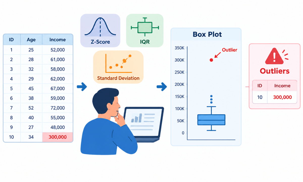
An outlier is a value that differs substantially from the rest of the observations. It may indicate a data-entry mistake, a measurement error, or a genuine but uncommon event.
For example, a product price entered as ₹500,000 instead of ₹5,000 could be an error. However, an unusually large order may be completely valid.
Two common outlier detection methods are the interquartile range (IQR) and the Z-score.
Interquartile range method
The IQR measures the spread of the middle 50% of the data.
IQR=Q3-Q1
Here, Q1 is the 25th percentile and Q3 is the 75th percentile. A common rule flags values below Q1-1.5IQR or above Q3+1.5IQR.
Use Python to identify these values:
Q1 = df["sales"].quantile(0.25)Q3 = df["sales"].quantile(0.75)IQR = Q3 - Q1lower_bound = Q1 - 1.5 * IQRupper_bound = Q3 + 1.5 * IQRoutliers = df[ (df["sales"] < lower_bound) | (df["sales"] > upper_bound)]print(outliers)
The IQR method is useful for exploratory data analysis, particularly when numerical data is skewed. However, it flags potential outliers rather than proving that a value is incorrect.
Z-score method
A Z-score measures how far a value is from the mean in standard deviation units.
z=x-
Here, x is the observation, is the mean, and is the standard deviation.
from scipy.stats import zscoredf["z_score"] = zscore( df["sales"], nan_policy="omit")outliers = df[df["z_score"].abs() > 3]
A common screening rule flags absolute Z-scores greater than 3. This approach works best when the distribution is reasonably close to normal. Extreme values can also affect the mean and standard deviation, making Z-scores less reliable for highly skewed data.
Use box plots and histograms alongside statistical rules to understand the distribution. Apponix's article on essential data cleaning tools and techniques provides additional context on common data preparation methods.
5. Handle Outliers Without Losing Important Information
After detecting potential outliers, decide whether to retain, correct, transform, cap, or remove them. The choice should reflect the reason behind each unusual value.
Correct errors and retain valid observations
If a value is clearly caused by a data-entry or measurement error, correct it using a verified source where possible. If the value represents a genuine event, retaining it may be essential.
For example, removing unusually high sales transactions could hide important business activity during a seasonal promotion.
Apply capping or winsorisation
Capping limits extreme observations to specified boundaries while retaining the records.
lower = df["sales"].quantile(0.01)upper = df["sales"].quantile(0.99)df["sales_capped"] = df["sales"].clip( lower=lower, upper=upper)
This example limits values to the first and 99th percentiles. It can reduce the influence of extreme values, but it also changes the original distribution. Compare results before and after capping to determine whether the change is justified.
Use transformations for skewed data
Log transformations can reduce right skew in positive numerical data.
df["log_sales"] = np.log1p(df["sales"])
The log1p() function calculates the natural logarithm of one plus the value. It can help when sales figures vary widely, although it does not automatically eliminate outliers.
For more background on preparing raw datasets, read Data Cleaning in Python: 10 Best Practices for Data Scientists.
6. Avoid Distorting Analysis and Machine Learning Models
Data cleaning decisions can affect statistical conclusions and predictive performance. A few precautions help preserve data quality.
-
Avoid blind deletion: Removing too many records can reduce sample size and introduce selection bias.
-
Preserve original values: Create cleaned columns or retain a copy of the source data for comparison and auditing.
-
Check distributions: Compare summary statistics, histograms, and box plots before and after treatment.
-
Prevent data leakage: For machine learning, fit imputation and outlier-treatment rules on the training data, then apply the same rules to validation and test data.
-
Consider business context: An unusual transaction or medical measurement may be more informative than an ordinary observation.
-
Document every change: Record the reason for each treatment, the method used, and its effect on the dataset.
Scikit-learn provides tools such as SimpleImputer, KNNImputer, and Pipeline to make data preprocessing more consistent and repeatable.
For example, a pipeline can impute missing numerical values using the training-set median before fitting a machine learning model:
from sklearn.impute import SimpleImputerfrom sklearn.pipeline import Pipelinefrom sklearn.preprocessing import StandardScalerfrom sklearn.linear_model import LinearRegressionpipeline = Pipeline([ ("imputer", SimpleImputer(strategy="median")), ("scaler", StandardScaler()), ("model", LinearRegression())])pipeline.fit(X_train, y_train)predictions = pipeline.predict(X_test)
Here, X_train, y_train, and X_test represent the training features, training target, and test features. The pipeline learns imputation and scaling parameters from the training data, helping prevent information from the test set from influencing model preparation.
Outlier treatment can also be incorporated into a suitable preprocessing pipeline when needed. Its method should be selected and validated according to the dataset and modelling objective.
7. Build a Repeatable Data Cleaning Workflow
A reliable workflow makes data preparation easier to maintain across projects. Instead of treating each problem separately, follow a consistent sequence:
-
Inspect: Review column names, data types, duplicates, and summary statistics.
-
Measure: Calculate missing-value percentages and identify potential outliers.
-
Investigate: Check data sources, collection methods, and domain-specific rules.
-
Treat: Apply suitable imputation, correction, transformation, or removal methods.
-
Validate: Compare distributions and summary statistics before and after cleaning.
-
Document: Record the decisions so the process can be reviewed and reproduced.
This workflow can be adapted to customer analytics, financial reporting, sales forecasting, and machine learning applications. It also creates a clear record of how raw data becomes suitable for analysis.
Conclusion
Handling missing values and outliers is an essential part of data preparation. Python libraries such as Pandas, NumPy, SciPy, and Scikit-learn provide practical methods to detect data-quality issues and apply suitable treatments.
The most important step is to understand why a value is missing or unusual before changing it. Mean and median imputation, IQR detection, Z-scores, capping, and transformations are useful techniques, but none should be applied without considering the data distribution and analytical objective.
Developing these skills requires practice with real datasets, statistical analysis, and machine learning workflows. Learners exploring these areas through a Data Science Course in Bangalore can use Python-based projects to understand how data cleaning decisions affect the quality of analysis and model predictions.
2)https://www.xgblog.ai/p/dealing-with-missing-values-part

Apponix Academy
Apponix Academy